Original Title:Game Theory on Polymarket: The 5 Formulas tested on 72 million trades, Author: Movez(@0xMovez)
Compiled | Odaily Planet Daily(@OdailyChina); Translator | Asher(@Asher_ 0210)
On the Las Vegas Strip, the average return rate of slot machines is about 93%, meaning for every dollar invested, you only get back an average of $0.93; on Polymarket, however, traders voluntarily accept returns as low as $0.43, using $1 to bet on outcomes with odds even worse than those in casinos.
This is not a metaphor, but based on real data. Researcher Jonathan Becker analyzed all settled markets on Kalshi, covering 72.1 million trades with a total volume of $18.26 billion. The patterns he discovered also apply to Polymarket—same mechanisms, same biases, meaning the same opportunities. The data's conclusion is straightforward: approximately 87% of prediction market wallets end up losing money, but the remaining 13% don't win by luck; they master a set of mathematical methods that most traders aren't even aware of.
This article will break down 5 game theory formulas that separate winners from losers, each accompanied by its mathematical principle, real-world examples, and runnable Python code. Some traders already applying these methods in practice include:
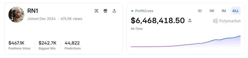
- RN (Polymarket address: https://polymarket.com/profile/%40rn1): A Polymarket algorithmic trading bot that has achieved over $6 million in total profit in sports markets based on the formulas in this article.
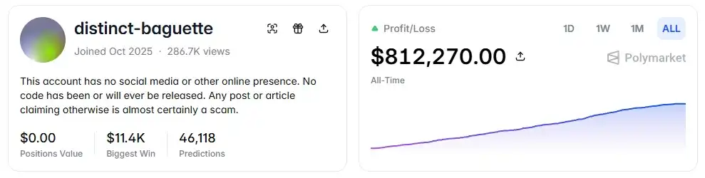
- distinct-baguette (Polymarket address: https://polymarket.com/profile/%40distinct-baguette): Turned $560 into $812,000 through market making in UP/DOWN markets.
I. Expected Value: The Core Formula
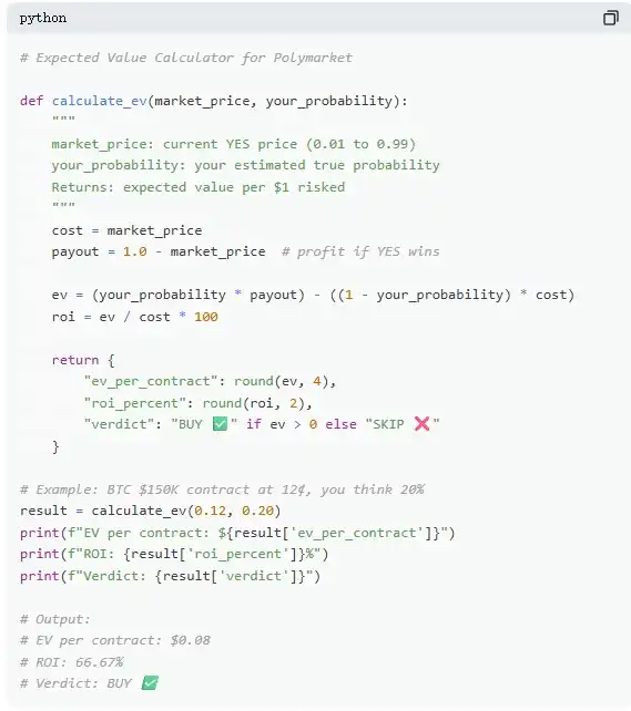
On Polymarket, every trade is essentially a judgment of expected value. Most traders rely on intuition, while the 13% of winners use mathematics to make decisions. Expected Value (EV) measures not a single outcome, but the average return over many repetitions, used to judge whether a trade is worth making.
Take a real market as an example: "Will Bitcoin reach $150,000 before June 2026?" The current YES price is 12¢, corresponding to a market-implied probability of 12%. If, based on on-chain data, halving cycles, and ETF flows, you judge the true probability to be around 20%, then this trade has positive expected value. According to this calculation, for every contract bought at 12¢, the long-term average gain is 8¢; buying 100 contracts, at a cost of $12, yields an expected profit of $8, a return of approximately +66.7%.
But the data shows that most prediction market traders do not perform such calculations. In a sample covering 72 million trades, takers (market buyers) lost an average of about 1.12% per trade, while makers (limit order placers) profited an average of about 1.12% per trade. The difference between them lies not in information, but in patience—makers wait for positive EV opportunities, while takers are more prone to impulsive trading.
II. Mispricing: The Low-Price Contract Trap
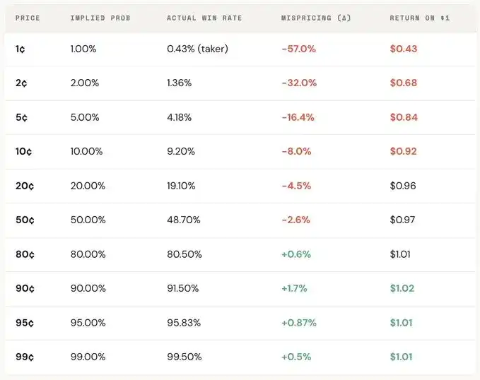
"Long-shot bias" is one of the most expensive mistakes in prediction markets. Traders often systematically overestimate low-probability events, paying too high a price for seemingly cheap contracts. A contract priced at 5¢ should have a 5% win rate theoretically, but on Kalshi the actual win rate is only 4.18%, corresponding to a -16.36% pricing偏差 (bias); in more extreme cases, a 1¢ contract should have a 1% win rate, but for takers, the actual win rate is only 0.43%, a偏差 of -57%.
Looking at the overall distribution, the market is relatively accurate in the middle range (30¢–70¢), but shows significant bias at the extremes: contracts below 20¢ generally have actual win rates lower than their price-implied probability; contracts above 80¢ often have win rates higher than their price-reflected probability.
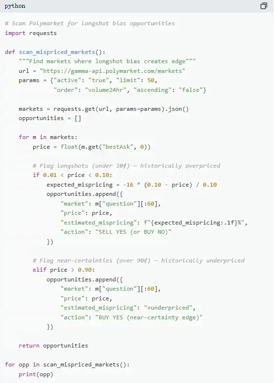
In other words, market inefficiency is concentrated at the extremes, and these intervals are precisely where emotional trading is most concentrated. Specifically, there are two formulas:
Formula 1: Mispricing (δ)
Mispricing measures the deviation between a contract's actual win rate and its implied probability. Taking the 5¢ contract as an example, across all settled markets, assume there were 100,000 trades executed at 5¢, of which 4,180最终 resulted in YES. The actual win rate is 4.18%, while the price implies a probability of 5.00%. The difference is -0.82 percentage points, a relative偏差 of approximately -16.36%. This means that for every 5¢ contract bought, you are effectively paying a premium of about 16.36%.
Formula 2: Gross Excess Return per Trade (ri)
If mispricing reflects the overall bias, then the gross excess return per trade reveals the actual return structure of each individual trade, and it is here that behavioral biases become clear. When buying a 5¢ contract, two outcomes are possible: if the contract hits, the gain can be +1900% (~20x return); if it misses, the loss is 100%, and the invested 5¢ goes to zero.
This is why the "long-shot bias" is so attractive—if it hits, the回报 is extremely high, easily remembered, amplified, and shared. But overall, its actual hit rate is lower than the probability implied by the price, and the asymmetric structure between "total loss" and "extremely high gain" creates negative expected value over many trades, essentially equivalent to buying overvalued lottery tickets.
Looking at the overall distribution, this bias has a clear price gradient: the lower the price, the worse the return. For example, as a taker, for every $1 invested in 1¢ contracts, you get back only about $0.43 on average; for 90¢ contracts, every $1 invested yields about $1.02 on average. The cheaper the price, the worse the actual trading conditions.
Further breaking down by role reveals an almost mirror-image relationship. The losses of takers in the low-price range (up to -57%) correspond almost exactly to the gains of makers in the same range; the overall market's pricing bias lies somewhere between the two. In other words, almost every cent lost by takers is gained by makers.
From a game theory perspective, low-probability contracts are usually systematically overestimated, while high-probability contracts are often underestimated. The real strategy is not to chase long-shots, but to sell them and buy high-certainty outcomes.
III. Kelly Criterion: How Much to Bet
When you find a trade with positive expected value, the real question just begins: how much should the trader bet? Bet too much, and one loss could wipe out weeks of gains; bet too little, and even with an edge, the growth is too slow to be meaningful. Between "all-in" and "not betting at all," there is a mathematically optimal betting fraction: the Kelly Criterion.
The Kelly Criterion was proposed by John Kelly Jr. in 1956, initially to optimize signal noise in communications, but later proven to be one of the most effective position sizing methods in gambling, trading, and even prediction markets. Professional poker players, sports betting experts, and Wall Street quant funds almost all use some form of Kelly strategy.

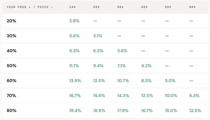
In prediction markets, since contracts are binary (resulting in $1 or $0) and the price itself represents probability, the application of the Kelly Criterion is more direct. The key is understanding the odds (b): if you buy a YES contract for 30¢, you are essentially risking $0.30 to win $0.70, corresponding to odds of 0.70 / 0.30 ≈ 2.33; at a price of 50¢, the odds are 1; at 10¢, 9; at 80¢, only 0.25. The higher the odds, the larger the bet fraction Kelly suggests, assuming an edge exists.
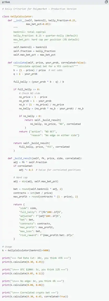
But a key principle is not to use Full Kelly. Although mathematically Full Kelly maximizes long-term growth rate, in practice its volatility is extreme, with drawdowns often exceeding 50%. It might have the highest returns over a very long period, but the intense volatility along the way often makes it difficult for most people to stick with. Therefore, a more common practice is to use Fractional Kelly (e.g., 1/2 or 1/4 Kelly). For example, under stable win rate conditions, Full Kelly, while ultimately having the highest equity curve, is very volatile; 1/4 Kelly grows more smoothly with controllable drawdowns; 1/2 Kelly falls somewhere in between.
Essentially, the Kelly Criterion provides a discipline: first determine if an edge exists (i.e., subjective probability is higher than market-implied probability), and on that basis, decide how much capital to commit. Only when both "whether to bet" and "how much to bet" are constrained by mathematics does trading truly move from gambling to strategy.
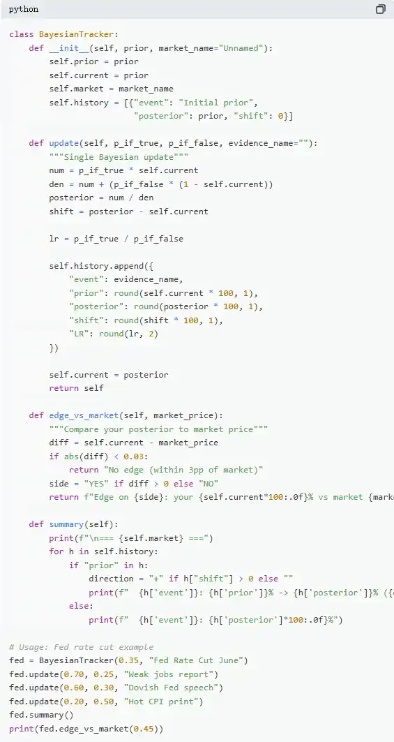
IV. Bayesian Updating: Changing Your Mind Like an Expert
Prediction markets fluctuate essentially because new information constantly enters. The key is not whether the initial judgment was correct, but how to adjust beliefs when evidence changes. Most traders either ignore new information or overreact, while Bayesian updating provides a mathematical method for "how much adjustment is reasonable."
Its core logic can be simply understood as new judgment = degree to which evidence supports the original hypothesis × original judgment ÷ overall probability of that evidence occurring. In practical application, it is usually expanded via the law of total probability to get a more calculable form.
Take a typical market: "Will the Fed cut rates at the June meeting?" The current market price is 35¢, corresponding to a 35% probability, serving as the initial belief (prior). Then the non-farm payroll data is released, showing only 120K new jobs (expected 200K), with rising unemployment and slowing wage growth. In this scenario, if the Fed were indeed going to cut rates, the probability of seeing weak employment data is high, estimated at 70%; if it were not going to cut rates, the probability of such data appearing is lower but still possible, estimated at 25%.
Substituting into Bayesian updating, the new (posterior) probability becomes approximately 60.1%, a one-time upward revision from 35% to 60.1%, an increase of about 25 percentage points. This means one key piece of information can significantly alter market judgment.
In practice, you don't need to calculate the full formula every time. A more common method is the "likelihood ratio." The same piece of information (e.g., LR = 3) has different impacts depending on the initial belief: starting from 10%, it might increase to about 25%; from 50%, to 75%; from 90%, to only about 96%. The higher the uncertainty, the greater the impact of information.
The traders who consistently outperform in prediction markets long-term are not necessarily those with the "most accurate" initial calls, but those who can adjust their judgments the fastest and most reasonably when new evidence appears. The Bayesian method essentially provides the scale for this "speed of adjustment."
V. Nash Equilibrium: The "Poker Formula" in Prediction Markets
In poker, bluffing is never a gut decision, but a strategy that can be precisely calculated. Theoretically, there is an optimal bluffing frequency; once you deviate, skilled opponents can exploit it. The same logic applies to prediction markets. On Polymarket, "bluffing" corresponds to contrarian trading—taking a position against the majority when market pricing is biased; while "folding" is akin to being a passive taker, continuously paying a premium for market sentiment.
On Polymarket, makers and takers form a similar adversarial relationship. Contrarian trading (against market consensus) is like "bluffing," while trend-following trading (following mainstream judgment) is like "value betting." From an equilibrium perspective, the market should make marginal participants indifferent between "being a maker" and "being a taker." This state corresponds to the Nash Equilibrium in prediction markets.
But this equilibrium is not fixed; it adjusts dynamically with changes in participant structure. Data shows that different market categories correspond to different optimal strategies: in areas with more rational information and efficient pricing (e.g., financial markets), the contrarian space is smaller; in areas with stronger emotions and more concentrated irrationality (e.g., entertainment, sports), the market is more prone to pricing biases, thus providing opportunities for contrarian trading.
More importantly, this equilibrium has also changed significantly over time. In the early days (2021–2023), takers were actually the profitable group, and the optimal strategy leaned towards active trading (taking). But after the trading volume explosion in Q4 2024, professional market makers entered in large numbers, the market structure changed, and the equilibrium strategy shifted towards being a maker (~65%–70%). This is a typical result of game theory: when the participant structure changes, the optimal strategy evolves accordingly. Strategies that were effective in a "novice environment" can quickly become ineffective against "professional opponents," and the market's "meta" thus constantly iterates.
Summary
87% of prediction market wallets end up losing money, not because the market is manipulated, but because these traders never actually do the math. They buy long-shot contracts at prices worse than slot machines, decide position sizes by feel, ignore new information, and pay for "optimistic sentiment" with every market order.
The 13% who consistently profit are not luckier; they use these 5 formulas as a complete methodology, forming a full process from judgment to execution, with each step built on top of 72.1 million real trades.
This window won't last forever. As professional market makers enter, bid-ask spreads are being compressed rapidly. In 2022, takers still had a ~+2.0% advantage; now it has turned into -1.12%.
The only question is, will you evolve with the market, or continue buying $1 lottery tickets for a $0.43 return.