In the process of creating @insidersdotbot, I had in-depth exchanges with many high-frequency market-making teams and arbitrage teams. One of the biggest demands was how to develop arbitrage strategies.

Our users, friends, and partners are all exploring the complex and multi-dimensional trading path of Polymarket arbitrage. If you are an active Twitter user, I believe you have come across tweets like "I made X amount of money from prediction markets through XX arbitrage strategy."

However, most articles oversimplify the underlying logic of arbitrage, making it seem like "I can do it too" or "just use Clawdbot to solve it," without explaining in detail how to systematically understand and develop your own arbitrage system.

If you want to understand how arbitrage tools on Polymarket make money, this article is the most comprehensive explanation I have seen so far.

Since the original English text contains many highly technical parts that require further research, I have restructured and supplemented it to help you understand all the key points with just this article, without needing to stop and look up additional information.

Polymarket Arbitrage Is Not a Simple Math Problem

You see a market on Polymarket:

YES price $0.62, NO price $0.33.

You think: 0.62 + 0.33 = 0.95, less than $1.00. There's an arbitrage opportunity! Buy both YES and NO for $0.95, and no matter the outcome, you get back $1.00, netting $0.05.

You are correct.

But the problem is—while you are still manually calculating this addition problem, quantitative systems are doing something completely different.

They are simultaneously scanning 17,218 conditions across 2^63 possible outcome combinations, finding all pricing contradictions in milliseconds. By the time you finish placing your two orders, the spread has already disappeared. The system has already found the same漏洞 in dozens of related markets, calculated the optimal position size considering order book depth and fees, executed all trades in parallel, and moved funds to the next opportunity. [1]

The gap is not just speed. It's mathematical infrastructure.

Chapter 1: Why "Addition" Is Not Enough—The Marginal Polytope Problem

The Single Market Fallacy

First, a simple example.

Market A: "Will Trump win the election in Pennsylvania?"

YES price $0.48, NO price $0.52. Sums to exactly $1.00.

Looks perfect, no arbitrage opportunity, right?

Wrong.

Add another market, and the problem emerges.

Now look at Market B: "Will the Republican Party win Pennsylvania by more than 5 percentage points?"

YES price $0.32, NO price $0.68. Also sums to $1.00.

Both markets individually appear "normal." But there is a logical dependency here:

The US presidential election is not a nationwide vote count but is decided state by state. Each state is an independent "battleground," Whoever gets more votes in that state wins all of that state's electoral votes (winner-takes-all). Trump is the Republican candidate. So "Republican win in Pennsylvania" and "Trump win in Pennsylvania"—are the same thing. If the Republican wins by more than 5 percentage points, it not only means Trump won Pennsylvania but won big.

In other words, Market B's YES (Republican landslide) is a subset of Market A's YES (Trump wins)—a landslide necessarily implies a win, but a win does not necessarily imply a landslide.

And this logical dependency creates an arbitrage opportunity.

It's like you're betting on two things—"Will it rain tomorrow?" and "Will there be a thunderstorm tomorrow?"

If there is a thunderstorm, it must be raining (thunderstorm is a subset of rain). So the price of "Thunderstorm YES" cannot be higher than the price of "Rain YES." If the market pricing violates this logic, you can simultaneously buy low and sell high, earning "risk-free profit." This is arbitrage.

Exponential Explosion: Why Brute Force Search Doesn't Work

For any market with n conditions, there are theoretically 2^n possible price combinations.

Sounds manageable? Look at a real case.

2010 NCAA Tournament Market [2]: 63 games, each with win/loss outcomes. The number of possible outcome combinations is 2^63 = 9,223,372,036,854,775,808—over 9.2 quintillion. There were over 5,000 markets.

How big is 2^63? If you check 1 billion combinations per second, it would take about 292 years to check them all. This is why "brute force search" is completely infeasible here.

Check each combination one by one? Computationally impossible.

Look at the 2024 US election. The research team found 1,576 pairs of potentially dependent markets. If each market pair has 10 conditions, then each pair requires checking 2^20 = 1,048,576 combinations. Multiply by 1,576 pairs. By the time your laptop finishes calculating, the election results would have long been announced.

Integer Programming: Using Constraints Instead of Enumeration

The solution used by quantitative systems is not "enumerate faster," but to not enumerate at all.

They use Integer Programming to describe "which outcomes are legal."

Consider a real example. Duke vs. Cornell game market: Each team has 7 markets (0 to 6 wins), totaling 14 conditions, 2^14 = 16,384 possible combinations.

But there is a constraint: They cannot both win more than 5 games because they would meet in the semifinals (only one can advance).

How does Integer Programming handle this? Three constraints are enough:

· Constraint 1: Exactly one of Duke's 7 markets is true (Duke can only have one final win count).

· Constraint 2: Exactly one of Cornell's 7 markets is true.

· Constraint 3: Duke wins 5 games + Duke wins 6 games + Cornell wins 5 games + Cornell wins 6 games ≤ 1 (They cannot both win that many).

Three linear constraints replace 16,384 brute force checks.

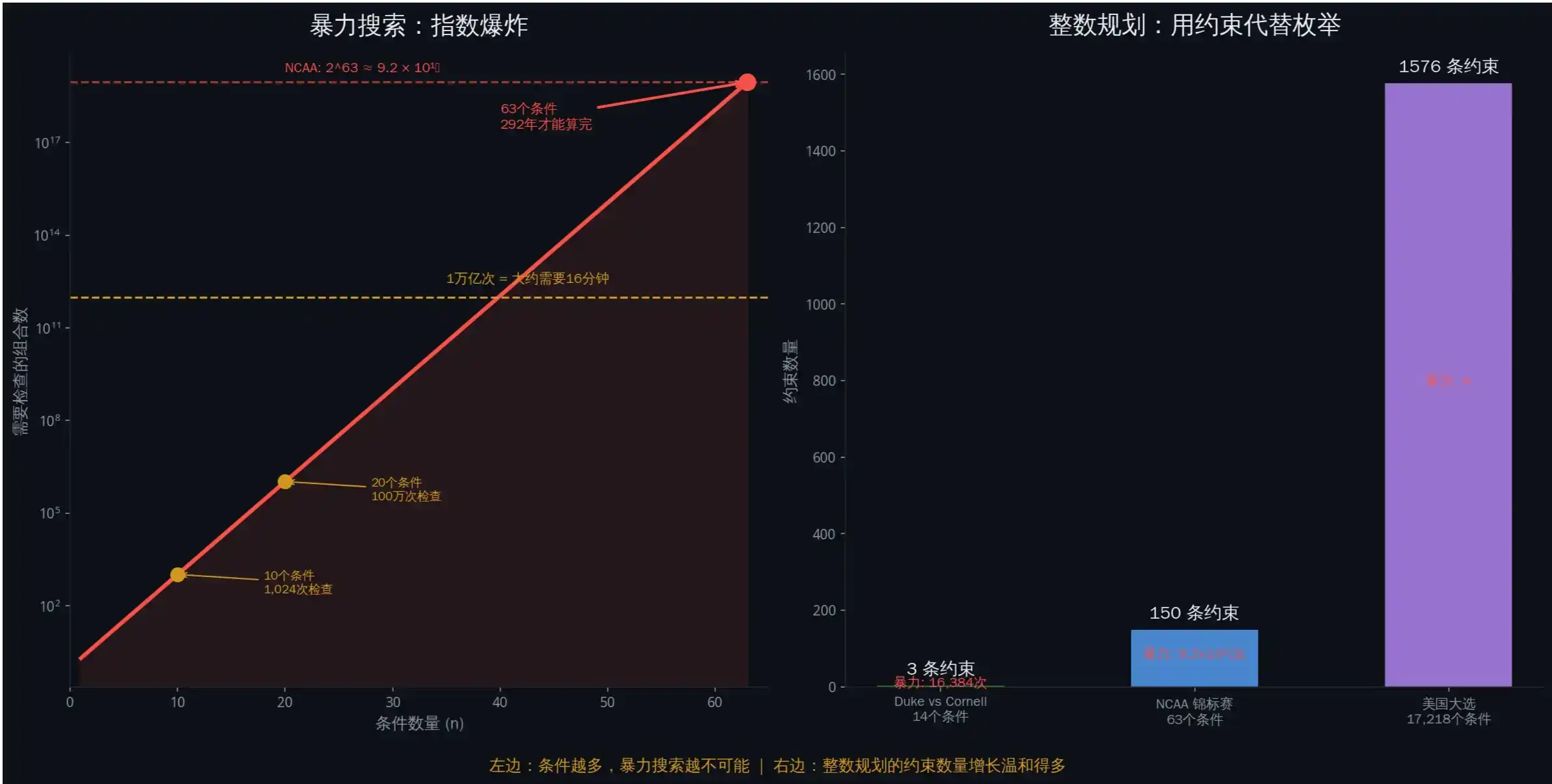
In other words, brute force search is like reading every word in the dictionary to find a specific word. Integer programming is like flipping directly to the page starting with that letter. You don't need to check all possibilities, you just need to describe "what a legal answer looks like," and then let the algorithm find pricing that violates the rules.

Real data: 41% of markets had arbitrage [2]

The original text mentions that the research team analyzed data from April 2024 to April 2025:

• Checked 17,218 conditions

• Among them, 7,051 conditions had single-market arbitrage (41%)

• Median pricing deviation: $0.60 (should be $1.00)

• 13 confirmed cross-market exploitable arbitrage pairs

A median deviation of $0.60 means the market frequently deviates by 40%. This is not "close to efficient"; this is "massively exploitable."

Chapter 2: Bregman Projection—How to Calculate the Optimal Arbitrage Trade

Discovering arbitrage is one problem. Calculating the optimal arbitrage trade is another.

You can't simply "take an average" or "adjust the price slightly." You need to project the current market state onto the arbitrage-free legal space while preserving the information structure within the prices.

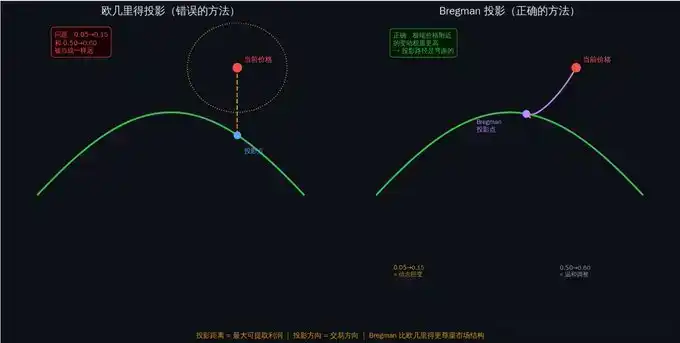
Why "Straight-Line Distance" Doesn't Work

The most intuitive idea: Find the "legal price" closest to the current price and trade the difference.

In mathematical terms, minimize the Euclidean distance: ||μ - θ||2

But this has a fatal flaw: It treats all price changes as the same.

A rise from $0.50 to $0.60, and a rise from $0.05 to $0.15, are both a 10-cent increase. But their information content is completely different.

Why? Because prices represent implied probabilities. A change from 50% to 60% is a moderate adjustment of view. A change from 5% to 15% is a massive shift in belief—an almost impossible event suddenly becomes "somewhat possible."

Imagine you are weighing yourself. Going from 70 kg to 80 kg, you say "gained a little weight." But going from 30 kg to 40 kg (if you are an adult), that's "from near death to severe malnutrition." The same 10 kg change has completely different significance. It's the same with prices—price changes closer to 0 or 1 carry more information.

Bregman Divergence: The Correct "Distance"

Polymarket's market makers use LMSR (Logarithmic Market Scoring Rule) [4], where prices essentially represent probability distributions.

In this structure, the correct distance measure is not Euclidean distance, but Bregman divergence. [5]

For LMSR, the Bregman divergence becomes the KL divergence (Kullback-Leibler divergence) [6]—a measure of the "information-theoretic distance" between two probability distributions.

You don't need to remember the formula. You just need to understand one thing:

KL divergence automatically gives higher weight to changes near extreme prices. A change from $0.05 to $0.15 is "further" in KL divergence than a change from $0.50 to $0.60. This aligns perfectly with our intuition—extreme price changes imply larger information shock.

A good example is the recent @zachxbt prediction market where Axiom overtook Meteora at the last moment, also marked by extreme price movements.

Arbitrage Profit = Distance of the Bregman Projection

This is one of the core conclusions referenced by the original author from the paper:

The maximum guaranteed profit obtainable from any trade equals the Bregman projection distance from the current market state to the arbitrage-free space.

In simpler terms: The further the market price deviates from the "legal space," the more money you can make. And the Bregman projection tells you:

1. What to buy and sell (the projection direction indicates the trade direction)

2. How much to buy and sell (considering order book depth)

3. How much you can earn (the projection distance is the maximum profit)

The top arbitrageur made $2,009,631.76 in a year. [2] His strategy was to solve this optimization problem faster and more accurately than everyone else.

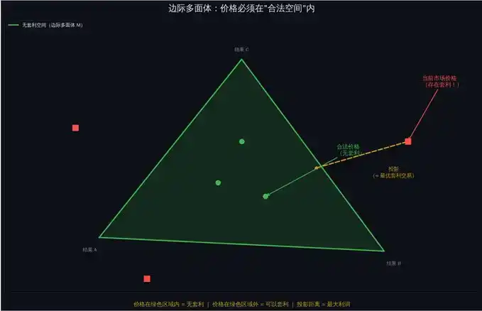
To use an analogy, imagine you are standing on a mountain, and there is a river at the foot (the arbitrage-free space). Your current location (current market price) is some distance from the river.

Bregman projection helps you find the "shortest path from your location to the river"—but not the straight-line distance, rather the shortest path considering the terrain (market structure). The length of this path is the maximum profit you can earn.

Chapter 3: Frank-Wolfe Algorithm—Turning Theory into Executable Code

Okay, now you know: To calculate optimal arbitrage, you need to perform a Bregman projection.

But the problem is—directly calculating the Bregman projection is infeasible.

Why? Because the arbitrage-free space (marginal polytope M) has an exponential number of vertices. Standard convex optimization methods require access to the full constraint set, meaning enumerating every legal outcome. We just said this is impossible at scale.

The Core Idea of Frank-Wolfe

The genius of the Frank-Wolfe algorithm [7] is: It doesn't try to solve the whole problem at once, but approaches the answer step by step.

It works like this:

Step 1: Start with a small set of known legal outcomes.

Step 2: Optimize over this small set to find the current optimal solution.

Step 3: Use integer programming to find a new legal outcome and add it to the set.

Step 4: Check if it's close enough to the optimal solution. If not, go back to Step 2.

Each iteration adds only one vertex to the set. Even after 100 iterations, you only need to track 100 vertices—not 2^63.

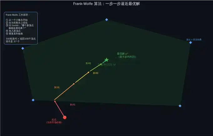
Imagine you are in a huge maze looking for the exit.

The brute force method is to walk every path. The Frank-Wolfe method is: First, take any path, then at each fork, ask a "guide" (integer programming solver): "From here, which direction is most likely to lead to the exit?" Then take a step in that direction. You don't need to explore the entire maze, just make the right choice at each key node.

Integer Programming Solver: The "Guide" for Each Step

Each iteration of Frank-Wolfe requires solving an integer linear programming problem. This is theoretically NP-hard (meaning "no known fast general algorithm exists").

But modern solvers, like Gurobi [8], can solve well-structured problems efficiently.

The research team used Gurobi 5.5. Actual solving times:

• Early iterations (few games finished): less than 1 second

• Mid-stage (30-40 games finished): 10-30 seconds

• Late stage (50+ games finished): less than 5 seconds

Why faster later? Because as game results are determined, the feasible solution space shrinks. Fewer variables, tighter constraints, faster solving.

Gradient Explosion Problem and Barrier Frank-Wolfe

Standard Frank-Wolfe has a technical problem: When the price approaches 0, the gradient of LMSR tends towards negative infinity. This causes algorithm instability.

The solution is Barrier Frank-Wolfe: Optimize not on the full polytope M, but on a slightly "contracted" version M. The contraction parameter ε adaptively decreases with iterations—starting farther from the boundary (stable), then gradually approaching the true boundary (accurate).

Research shows that 50 to 150 iterations are sufficient for convergence in practice.

Real Performance

A key finding in the paper [2]:

In the first 16 games of the NCAA tournament, Frank-Wolfe Market Maker (FWMM) and simple Linear Constraint Market Maker (LCMM) performed similarly—because the integer programming solver was still too slow.

But after 45 games were finished, the first successful 30-minute projection was completed.

From then on, FWMM was 38% better than LCMM at pricing the markets.

The turning point was: when the outcome space shrank enough for integer programming to complete solving within the trading time frame.

FWMM is like a student warming up in the first half of the exam but once in form, starts crushing it. LCMM is the student performing steadily but with a limited ceiling. The key difference: FWMM has a stronger "weapon" (Bregman projection), it just needs time to "load" (wait for the solver to finish).

Chapter 4: Execution—Why You Might Still Lose Money Even After Calculating

You detected arbitrage. You calculated the optimal trade using Bregman projection.

Now you need to execute.

This is where most strategies fail.

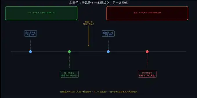
Non-Atomic Execution Problem

Polymarket uses a CLOB (Central Limit Order Book) [9]. Unlike decentralized exchanges, trades on a CLOB are executed sequentially—you cannot guarantee all orders will fill simultaneously.

Your arbitrage plan:

Buy YES, price $0.30. Buy NO, price $0.30. Total cost $0.60. Regardless of outcome, get back $1.00. Profit $0.40.

Reality:

· Submit YES order → Filled at $0.30 ✓

· Your order changed the market price.

· Submit NO order → Filled at $0.78 ✗

· Total cost: $1.08. Return: $1.00. Actual result: Loss of $0.08.

One leg filled, the other didn't. You are exposed.

This is why the paper only counted opportunities with a profit margin exceeding $0.05. Smaller spreads get eaten by execution risk.

VWAP: The Real Execution Price

Don't assume you can trade at the quoted price. Calculate the Volume-Weighted Average Price (VWAP) [10].

The research team's method: For each block on the Polygon chain (about 2 seconds), calculate the VWAP of all YES trades and the VWAP of all NO trades in that block. If |VWAP_yes + VWAP_no - 1.0| > 0.02, record it as an arbitrage opportunity [2].

VWAP is the "average price you actually pay." If you want to buy 10,000 tokens, but the order book has only 2,000 at $0.30, 3,000 at $0.32, and 5,000 at $0.35—your VWAP is (2000×0.30 + 3000×0.32 + 5000×0.35) / 10000 = $0.326. Significantly more expensive than the "best price" of $0.30 you saw.

Liquidity Constraints: How Much You Can Earn Depends on Order Book Depth

Even if the price is indeed mispriced, the profit you can earn is limited by the available liquidity.

Real example [2]:

Market shows arbitrage: Sum of YES prices = $0.85. Potential profit: $0.15 per dollar. But the order book depth at these prices is only $234. Maximum extractable profit: $234 × 0.15 = $35.10.

For cross-market arbitrage, you need liquidity on all legs simultaneously. The smallest one determines your upper limit.

This is also why, in existing quantitative platforms, showing the impact of order price on execution price is crucial.

Chapter 5: The Complete System—What Was Actually Deployed

Theory is clean. Production is messy.

This is what a truly operational arbitrage system looks like [2].

Data Pipeline

Real-time data: WebSocket connection to Polymarket's API [9], receiving order book updates (price/quantity changes), trade pushes, market creation/settlement events.

Historical data: Query contract events via Alchemy Polygon node API—OrderFilled (trade execution), PositionSplit (new token minting), PositionsMerge (token burning).

The research team analyzed 86 million trades [2]. This scale requires infrastructure, not scripts.

There are also plans to open-source a high-speed trading API. If you plan to use a similar trading model and hope to experience the API firsthand, feel free to DM me anytime.

Dependency Detection Layer

For the 305 US election markets, there were 46,360 possible pairs to check. Manual analysis is impossible.

The research team used a clever method: Using the DeepSeek-R1-Distill-Qwen-32B large language model for initial screening.

Input: Descriptions of two market conditions. Output: JSON of legal outcome combinations.

Then perform three layers of verification: Does each market have exactly one condition true? Is the number of legal combinations less than n × m (indicating dependency)? Does the dependency subset satisfy arbitrage conditions?

Result: 40,057 pairs independent (no arbitrage) → 1,576 pairs had dependencies (potential arbitrage) → 374 pairs met strict conditions → 13 pairs verified exploitable by manual check [2].

The LLM's accuracy on complex multi-condition markets was 81.45%. Good enough for initial screening, but requires manual verification before execution.

Three-Tier Optimization Engine

· Tier 1: Simple Linear Constraints (LCMM). Quick check of basic rules—"sum of probabilities equals 1", "if A implies B, then P(A) cannot exceed P(B)". Completes in milliseconds, removes obvious pricing errors.

· Tier 2: Integer Programming Projection (Frank-Wolfe + Gurobi). This is the core. Parameters: Alpha = 0.9 (extract at least 90% of available arbitrage), initial ε = 0.1 (10% contraction), convergence threshold = 1e-6, time limit = 30 minutes. Typical iterations: 50-150. Solving time per iteration: 1-30 seconds.

· Tier 3: Execution Verification. Before submitting orders, simulate execution on the current order book. Check: Is liquidity sufficient? What is the expected slippage? What is the guaranteed profit after deducting slippage? Is the profit above the minimum threshold ($0.05)? Execute only if all pass.

Position Management: Modified Kelly Criterion

The standard Kelly Criterion [11] tells you what fraction of your capital to invest in a trade. But in arbitrage scenarios, an adjustment for execution risk is needed:

f = (b×p - q) / b × √p

Where b is the arbitrage profit percentage, p is the probability of full execution (estimated based on order book depth), q = 1 - p.

Upper limit: 50% of the order book depth. Beyond this proportion, your order itself will significantly move the market.

Final Results

From April 2024 to April 2025, total extracted profit:

Single Condition Arbitrage: Buy both sides low $5,899,287 + Sell both sides high $4,682,075 = $10,581,362

Market Rebalancing: Buy all YES low $11,092,286 + Sell all YES high $612,189 + Buy all NO $17,307,114 = $29,011,589

Cross-Market Combination Arbitrage: $95,634

Total: $39,688,585

The top 10 arbitrageurs took $8,127,849 (20.5% of the total). The top arbitrageur: $2,009,632, from 4,049 trades, average $496 per trade [2].

Not a lottery. Not luck. Systematic execution of mathematical precision.

The Final Reality

While traders are still reading "10 Tips for Prediction Markets," what are quantitative systems doing?

They are using integer programming to detect dependencies among 17,218 conditions. They are using Bregman projection to calculate optimal arbitrage trades. They are running the Frank-Wolfe algorithm to handle gradient explosions. They are using VWAP to estimate slippage and execute orders in parallel. They are systematically extracting $40 million in guaranteed profits.

The gap is not luck. It's mathematical infrastructure.

The paper is public [1]. The algorithms are known. The profits are real.

The question is: Can you build it before the next $40 million is extracted?

Concept Quick Reference

• Marginal Polytope → The space formed by all "legal prices." Prices must be within this space to be arbitrage-free. Can be understood as the "legal region for prices".

• Integer Programming → Using linear constraints to describe legal outcomes, avoiding brute force enumeration. Compresses 2^63 checks into a few constraints [3].

• Bregman Divergence / KL Divergence → Methods to measure the "distance" between two probability distributions, more suitable for price/probability scenarios than Euclidean distance. Gives higher weight to changes near extreme prices [5][6].

• LMSR (Logarithmic Market Scoring Rule) → The pricing mechanism used by Polymarket market makers, where prices represent implied probabilities [4].

• Frank-Wolfe Algorithm → An iterative optimization algorithm that adds only one new vertex per round, avoiding enumeration of exponentially many legal outcomes [7].

• Gurobi → An industry-leading integer programming solver, the "guide" for each Frank-Wolfe iteration [8].

• CLOB (Central Limit Order Book) → Polymarket's trade matching mechanism, orders execute sequentially, atomicity not guaranteed [9].

• VWAP (Volume-Weighted Average Price) → The average price you actually pay, considering order book depth. More realistic than "best quote" [10].

• Kelly Criterion → Tells you what fraction of your capital to invest in a trade, balancing return and risk [11].

• Non-Atomic Execution → The problem that multiple orders cannot be guaranteed to fill simultaneously. One leg fills, the other doesn't = exposure risk.

• DeepSeek → The large language model used for initial screening of market dependencies, accuracy 81.45%.