前言
书接上回,关于《用多因子模型构建强大的加密资产投资组合》系列文章中,我们已经发布了两篇:《理论基础篇》、《数据预处理篇》
本篇是第三篇:因子有效性检验。
在求出具体的因子值后,需要先对因子进行有效性检验,筛选符合显著性、稳定性、单调性、收益率要求的因子;因子有效性检验通过分析本期因子值与预期收益率的关系,从而确定因子的有效性。主要有 3 种经典方法:
IC / IR 法:IC / IR 值为因子值与预期收益率的相关系数,越大因子表现越好。
T 值(回归法):T 值体现下期收益率对本期因子值线性回归后系数的显著性,通过比较该回归系数是否通过 t 检验,来判断本期因子值对下期收益率的贡献程度,通常用于多元(即多因子)回归模型。
分层回测法:分层回测法基于因子值对 token 分层,再计算每层 token 的收益率,从而判断因子的单调性
一、IC / IR 法
(1)IC / IR 的定义
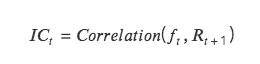
IC:即信息系数 Information Coefficient,代表因子预测 Tokens 收益的能力。某一期 IC 值为本期因子值和下期收益率的相关系数。
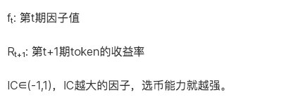
IC 越接近 1 ,说明因子值和下期收益率的正相关性越强,IC= 1 ,表示该因子选币 100% 准确,对应的是排名分最高的 token,选出来的 token 在下个调仓周期中,涨幅最大;
IC 越接近-1 ,说明因子值和下期收益率的负相关性越强,如果 IC=-1 ,则代表排名分最高的 token,在下个调仓周期中,跌幅最大,是一个完全反指的指标;
若 IC 越接近 0 ,则说明该因子的预测能力极其弱,表明该因子对于 token 没有任何的预测能力。
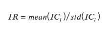
IR:信息比率 information ratio,代表因子获取稳定 Alpha 的能力。IR 为所有期 IC 均值除以所有期 IC 标准差。
当 IC 的绝对值大于 0.05 (0.02) 时,因子的选股能力较强。当 IR 大于 0.5 时,因子稳定获取超额收益能力较强。
(2)IC 的计算方式
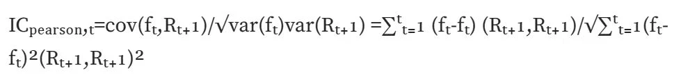
Normal IC (Pearson correlation):计算皮尔森相关系数,最经典的一种相关系数。但该计算方式存在较多假设前提:数据连续,正态分布,两个变量满足线性关系等等。
Rank IC (Spearman's rank coefficient of correlation):计算斯皮尔曼秩相关系数,先对两个变量排序,再根据排序后的结果求皮尔森相关系数。斯皮尔曼秩相关系数评估的是两个变量之间的单调关系,并且由于转换为排序值,受数据异常值影响较小;而皮尔森相关系数评估的是两个变量之间的线性关系,不仅对原始数据有一定的前提条件,并且受数据异常值影响较大。在现实计算中,求 rank IC 更符合。
(3)IC / IR 法代码实现
创建一个按日期时间升序排列的唯一日期时间值的列表--记录调仓日期 def choosedate(dateList, cycle)
class TestAlpha(object):
def __init__(self, ini_data):
self.ini_data = ini_data
def chooseDate(self, cycle, start_date, end_date):
'''
cycle: day, month, quarter, year
df: 原始数据框 df,date 列的处理
'''
chooseDate = []
dateList = sorted(self.ini_data[self.ini_data['date'].between(start_date, end_date)]['date'].drop_duplicates().values)
dateList = pd.to_datetime(dateList)
for i in range(len(dateList)-1):
if getattr(dateList[i], cycle) != getattr(dateList[i + 1 ], cycle):
chooseDate.append(dateList[i])
chooseDate.append(dateList[-1 ])
chooseDate = [date.strftime('%Y-%m-%d') for date in chooseDate]
return chooseDate
def ICIR(self, chooseDate, factor):
# 1.先展示每个调仓日期的 IC,即 ICt
testIC = pd.DataFrame(index=chooseDate, columns=['normalIC','rankIC'])
dfFactor = self.ini_data[self.ini_data['date'].isin(chooseDate)][['date','name','price', factor]]
for i in range(len(chooseDate)-1):
# ( 1) normalIC
X = dfFactor[dfFactor['date'] == chooseDate[i]][['date','name','price', factor]].rename(columns={'price':'close 0'})
Y = pd.merge(X, dfFactor[dfFactor['date'] == chooseDate[i+ 1 ]][['date','name','price']], on=['name']).rename(columns={'price':'close 1'})
Y['returnM'] = (Y['close 1'] - Y['close 0']) / Y['close 0']
Yt = np.array(Y['returnM'])
Xt = np.array(Y[factor])
Y_mean = Y['returnM'].mean()
X_mean = Y[factor].mean()
num = np.sum((Xt-X_mean)*(Yt-Y_mean))
den = np.sqrt(np.sum((Xt-X_mean)** 2)*np.sum((Yt-Y_mean)** 2))
normalIC = num / den # pearson correlation
# ( 2) rankIC
Yr = Y['returnM'].rank()
Xr = Y[factor].rank()
rankIC = Yr.corr(Xr)
testIC.iloc[i] = normalIC, rankIC
testIC =testIC[:-1 ]
# 2.基于 ICt,求['IC_Mean', 'IC_Std','IR','IC<0 占比--因子方向','|IC|>0.05 比例']
'''
ICmean: |IC|>0.05, 因子的选币能力较强,因子值与下期收益率相关性高。|IC|<0.05,因子的选币能力较弱,因子值与下期收益率相关性低
IR: |IR|>0.5,因子选币能力较强, IC 值较稳定。|IR|<0.5, IR 值偏小,因子不太有效。若接近 0,基本无效
IClZero(IC less than Zero): IC<0 占比接近一半->因子中性.IC>0 超过一大半,为负向因子,即因子值增加,收益率降低
ICALzpF(IC abs large than zero poin five): |IC|>0.05 比例偏高,说明因子大部分有效
'''
IR = testIC.mean()/testIC.std()
IClZero = testIC[testIC<0 ].count()/testIC.count()
ICALzpF = testIC[abs(testIC)>0.05 ].count()/testIC.count()
combined =pd.concat([testIC.mean(), testIC.std(), IR, IClZero, ICALzpF], axis= 1)
combined.columns = ['ICmean','ICstd','IR','IClZero','ICALzpF']
# 3.IC 调仓期内 IC 的累积图
print("Test IC Table:")
print(testIC)
print("Result:")
print('normal Skewness:', combined['normalIC'].skew(),'rank Skewness:', combined['rankIC'].skew())
print('normal Skewness:', combined['normalIC'].kurt(),'rank Skewness:', combined['rankIC'].kurt())
return combined, testIC.cumsum().plot()
二、T 值检验(回归法)
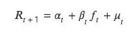
T 值法同样检验本期因子值和下期收益率关系,但与 ICIR 法分析二者的相关性不同,t 值法将下期收益率作为因变量 Y,本期因子值作为自变量 X,由 Y 对 X 回归,对回归出因子值的回归系数进行 t 检验,检验其是否显著异于 0 ,即本期因子是否影响下期收益率。
该方法本质是对双变量回归模型的求解,具体公式如下:

(1)回归法理论
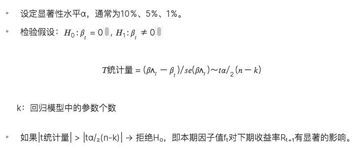
(2)回归法代码实现
def regT(self, chooseDate, factor, return_ 24 h):
testT = pd.DataFrame(index=chooseDate, columns=['coef','T'])
for i in range(len(chooseDate)-1):
X = self.ini_data[self.ini_data['date'] == chooseDate[i]][factor].values
Y = self.ini_data[self.ini_data['date'] == chooseDate[i+ 1 ]][return_ 24 h].values
b, intc = np.polyfit(X, Y, 1) # 斜率
ut = Y - (b * X + intc)
# 求 t 值 t = (\hat{b} - b) / se(b)
n = len(X)
dof = n - 2 # 自由度
std_b = np.sqrt(np.sum(ut** 2) / dof)
t_stat = b / std_b
testT.iloc[i] = b, t_stat
testT = testT[:-1 ]
testT_mean = testT['T'].abs().mean()
testT L1 96 = len(testT[testT['T'].abs() > 1.96 ]) / len(testT)
print('testT_mean:', testT_mean)
print('T 值大于 1.96 的占比:', testT L1 96)
return testT
三、分层回测法
分层指对所有 token 分层,回测指计算每层 token 组合的收益率。
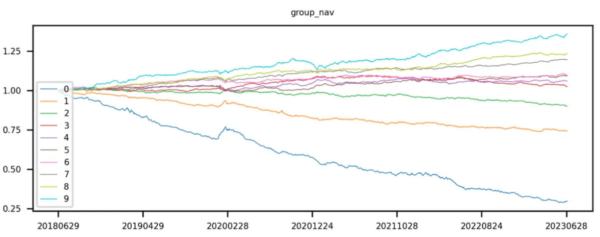
(1)分层
首先获取 token 池对应的因子值,通过因子值对 token 进行排序。升序排序,即因子值较小的排在前面,根据排序对 token 进行等分。第 0 层 token 的因子值最小,第 9 层 token 的的因子值最大。
理论上“等分”是指均等分拆 token 的个数,即每层 token 个数相同,借助分位数实现。现实中 token 总数不一定是层数的倍数,即每层 token 个数不一定相等。
(2)回测
将 token 按因子值升序分完 10 组后,开始计算每组 token 组合的收益率。该步骤将每层的 token 当成一个投资组合(不同回测期,每层的 token 组合所含的 token 都会有变化),并计算该组合整体的下期收益率。ICIR、t 值分析的是当期因子值和下期整体的收益率,但分层回测需要计算回测时间内每个交易日的分层组合收益率。由于有很多回测期有很多期,在每一期都需要进行分层和回测。最后对每一层的 token 收益率进行累乘,计算出 token 组合的累积收益率。
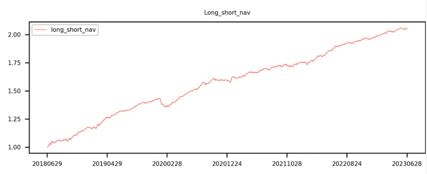
理想状态下,一个好的因子,第 9 组的曲线收益最高,第 0 组的曲线收益最低。
第 9 组减去第 0 组(即多空收益)曲线呈现单调递增。
(3)分层回测法代码实现
def layBackTest(self, chooseDate, factor):
f = {}
returnM = {}
for i in range(len(chooseDate)-1):
df 1 = self.ini_data[self.ini_data['date'] == chooseDate[i]].rename(columns={'price':'close 0'})
Y = pd.merge(df 1, self.ini_data[self.ini_data['date'] == chooseDate[i+ 1 ]][['date','name','price']], left_on=['name'], right_on=['name']).rename(columns={'price':'close 1'})
f[i] = Y[factor]
returnM[i] = Y['close 1'] / Y['close 0'] -1
labels = ['0','1','2','3','4','5','6','7','8','9']
res = pd.DataFrame(index=['0','1','2','3','4','5','6','7','8','9','LongShort'])
res[chooseDate[ 0 ]] = 1
for i in range(len(chooseDate)-1):
dfM = pd.DataFrame({'factor':f[i],'returnM':returnM[i]})
dfM['group'] = pd.qcut(dfM['factor'], 10, labels=labels)
dfGM = dfM.groupby('group').mean()[['returnM']]
dfGM.loc['LongShort'] = dfGM.loc['0']- dfGM.loc['9']res[chooseDate[i+ 1 ]] = res[chooseDate[ 0 ]] * ( 1 + dfGM['returnM']) data = pd.DataFrame({'分层累积收益率':res.iloc[: 10,-1 ],'Group':[ 0, 1, 2, 3, 4, 5, 6, 7, 8, 9 ]})
df 3 = data.corr()
print("Correlation Matrix:")
print(df 3)
return res.T.plot(title='Group backtest net worth curve')